By M. Tim Jones
Algorithms used in machine learning fall roughly into three categories: supervised, unsupervised, and reinforcement learning. Supervised learning involves feedback to indicate when a prediction is right or wrong, whereas unsupervised learning involves no response: The algorithm simply tries to categorize data based on its hidden structure. Reinforcement learning is similar to supervised learning in that it receives feedback, but it’s not necessarily for each input or state. This tutorial explores the ideas behind these learning models and some key algorithms used for each.
Machine-learning algorithms continue to grow and evolve. In most cases, however, algorithms tend to settle into one of three models for learning. The models exist to adjust automatically in some way to improve their operation or behavior.
Figure 1. Three learning models for algorithms
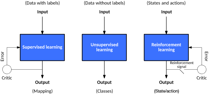
In supervised learning, a data set includes its desired outputs (or labels) such that a function can calculate an error for a given prediction. The supervision comes when a prediction is made and an error produced (actual vs. desired) to alter the function and learn the mapping.
In unsupervised learning, a data set doesn’t include a desired output; therefore, there’s no way to supervise the function. Instead, the function attempts to segment the data set into “classes” so that each class contains a portion of the data set with common features.
Finally, in reinforcement learning, the algorithm attempts to learn actions for a given set of states that lead to a goal state. An error is provided not after each example (as is the case for supervised learning) but instead on receipt of a reinforcement signal (such as reaching the goal state). This behavior is similar to human learning, where feedback isn’t necessarily provided for all actions but when a reward is warranted.
Now, let’s dig into each model and examine their approaches and key algorithms.
Supervised learning
Supervised learning is the simplest of the learning models to understand. Learning in the supervised model entails creating a function that can be trained by using a training data set, then applied to unseen data to meet some predictive performance. The goal is to build the function so that it generalizes well over data it has never seen.
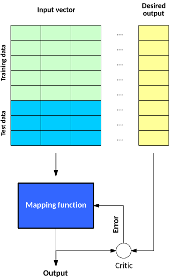
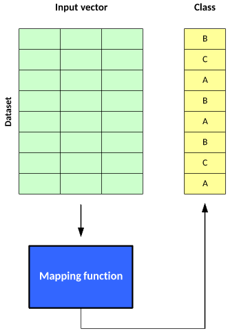
You build and test a mapping function with supervised learning in two phases (see image below). In the first phase, you segment a data set into two types of samples: training data and test data. Both training and test data contain a test vector (the inputs) and one or more known desired output values. You train the mapping function with the training data set until it meets some level of performance (a metric for how accurately the mapping function maps the training data to the associated desired output). In the context of supervised learning, this occurs with each training sample, where you use the error (actual vs. desired output) to alter the mapping function. In the next phase, you test the trained mapping function against the test data. The test data represents data that has not been used for training and provides a good measure for how well the mapping function generalizes to unseen data.
Figure 2. The two phases of building and testing a mapping function with supervised learning
Numerous algorithms exist under the supervised learning umbrella, such as support vector machines and naïve Bayes. Let’s look at two key approaches: neural networks and decision trees.
Neural networks
A neural network processes an input vector to a resulting output vector through a model inspired by neurons and their connectivity in the brain. The model consists of layers of neurons interconnected through weights that alter the importance of certain inputs over others. Each neuron includes an activation function that determines the output of the neuron (as a function of its input vector multiplied by its weight vector). The output is computed by applying the input vector to the input layer of the network, then computing the outputs of each neuron through the network (in a feed-forward fashion).
Figure 3. Layers of a typical neural network
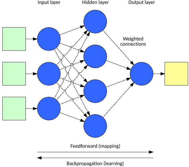
One of the most popular supervised learning methods for neural networks is called back-propagation. In back-propagation, you apply an input vector and compute the output vector. The error is computed (actual vs. desired), then back-propagated to adjust the weights and biases starting from the output layer to the input layer (as a function of their contribution to the output, adjusting for a learning rate). You can learn more about neural networks and back-propagation in “A neural networks deep dive.”
Decision trees
A decision tree is a supervised learning method for classification. Algorithms of this variety create trees that predict the result of an input vector based on decision rules inferred from the features present in the data. Decision trees are useful because they’re easy to visualize so you can understand the factors that lead to a result.
Figure 4. A typical decision tree
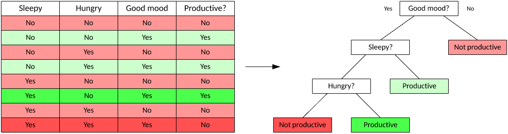
Two types of models exist for decision trees: classification trees, where the target variable is a discrete value and the leaves represent class labels (as shown in the example tree), and regression trees, where the target variable can take continuous values. You use a data set to train the tree, which then builds a model from the data. You can then use the tree for decision-making with unseen data (by walking down the tree based on the current test vector until a leaf is encountered).
Numerous algorithms exist for decision tree learning. One of the earliest was the Iterative Dichotomiser 3 (ID3), which works by splitting the data set into two separate data sets based on a single field in the vector. You select this field by calculating its entropy (a measure of the distribution of the values for that field). The goal is to select a field from the vector that will result in a decrease in entropy in subsequent splits of the data set as the tree is built.
Beyond ID3 is an improved algorithm called C4.5 (a successor of ID3) and Multivariate Adaptive Regression Splines (MARS), which builds decision trees with improved numerical data handling.
Unsupervised learning
Unsupervised learning is also a relatively simple learning model, but as the name suggests, it lacks a critic and has no way to measure its performance. The goal is to build a mapping function that categorizes the data into classes based on features hidden within the data.
As with supervised learning, you use unsupervised learning in two phases. In the first phase, the mapping function segments a data set into classes. Each input vector becomes part of a class, but the algorithm cannot apply labels to those classes.
Figure 5. The two phases of using unsupervised learning
The segmentation of the data into classes may be the result (from which you can then draw conclusions about the resulting classes), but you can use these classes further depending on the application. One such application is a recommendation system, where the input vector may represent the characteristics or purchases of a user, and users within a class represent those with similar interests who can then be used for marketing or product recommendations.
You can implement unsupervised learning by using a variety of algorithms, such as k-means clustering or adaptive resonance theory, or ART (a family of algorithms that implement unsupervised clustering of a data set).
K-means clustering
k-means clustering is a simple and popular clustering algorithm that originated in signal processing. The goal of the algorithm is to partition examples from a data set into k clusters. Each example is a numerical vector that allows the distance between vectors to be calculated as a Euclidean distance.
The simple example below visualizes the partitioning of data into k = 2 clusters, where the Euclidean distance between examples is smallest to the centroid (center) of the cluster, which indicates its membership.
Figure 6. Simple example of k-means clustering
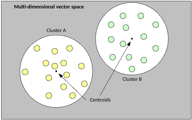
The k-means algorithm is extremely simple to understand and implement. You begin by randomly assigning each example from the data set into a cluster, calculate the centroid of the clusters as the mean of all member examples, then iterate the data set to determine whether an example is closer to the member cluster or the alternate cluster (given that k = 2). If the member is closer to the alternate cluster, the example is moved to the new cluster and its centroid recalculated. This process continues until no example moves to the alternate cluster.
As illustrated, k-means partitions the example data set into k clusters without any understanding of the features within the example vectors (that is, without supervision).
Adaptive resonance theory
Adaptive resonance theory (ART) is a family of algorithms that provide pattern recognition and prediction capabilities. You can divide ART along unsupervised and supervised models, but I focus here on the unsupervised side. ART is a self-organizing neural network architecture. The approach allows learning new mappings while maintaining existing knowledge.
Like k-means, you can use ART1 for clustering, but it has a key advantage in that rather than defining k at runtime, ART1 can alter the number of clusters based on the data.
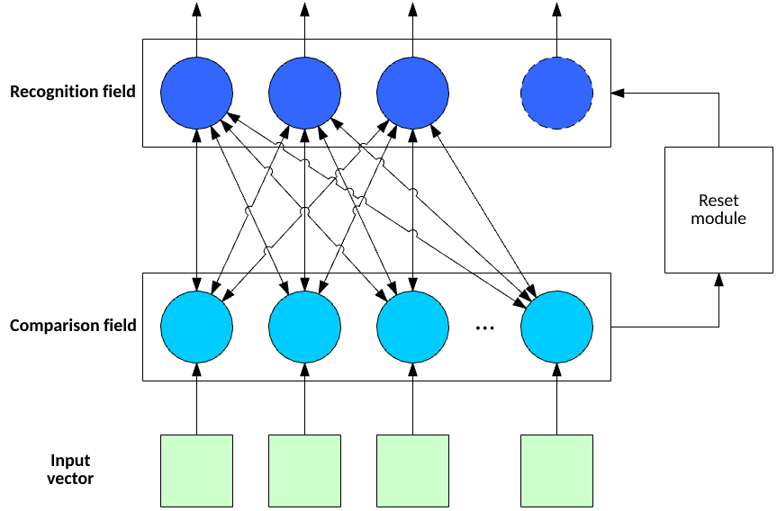
ART1 includes three key features: a comparison field (used to determine how a new feature vector fits within the existing categories), a recognition field (contains neurons that represent the active clusters), and a reset module. When the input vector is applied, the comparison field identifies the cluster in which it most closely fits. If the input vector matches in the recognition field above a vigilance parameter, then the connections to the neuron in the recognition field are updated to account for this new vector. Otherwise, a new neuron is created in the recognition field to account for a new cluster. When a new neuron is created, the existing neuron weights are not updated, allowing them to retain the existing knowledge. All examples of the data set are applied in this way until no example input vector changes cluster. At this point, training is complete.
Figure 7. Features of ART1
ART includes several algorithms that support binary input vectors or real-valued vectors (ART2). Predictive ART is a variation of ART1/2 but relies on supervised training.
Reinforcement learning
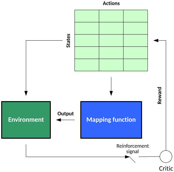
Reinforcement learning is an interesting learning model, with the ability not just to learn how to map an input to an output but to map a series of inputs to outputs with dependencies (Markov decision processes, for example). Reinforcement learning exists in the context of states in an environment and the actions possible at a given state. During the learning process, the algorithm randomly explores the state–action pairs within some environment (to build a state–action pair table), then in practice of the learned information exploits the state–action pair rewards to choose the best action for a given state that lead to some goal state. You can learn more about reinforcement learning in “Train a software agent to behave rationally with reinforcement learning.”
Figure 8. The reinforcement learning model
Consider a simple agent that plays blackjack. The states represent the sum of the cards for the player. The actions represent what a blackjack-playing agent may do — in this case, hit or stand. Training an agent to play blackjack would involve many hands of poker, where reward for a given state–action nexus is given for winning or losing. For example, the value for a state of 10 would be 1.0 for hit and 0.0 for stand (indicating that hit is the optimal choice). For state 20, the learned reward would likely be 0.0 for hit and 1.0 for stand. For a less-straightforward hand, a state of 17 may have action values of 0.95 stand and 0.05 hit. This agent would then probabilistically stand 95 percent of the time and hit 5 percent of the time. These rewards would be leaned over many hands of poker, indicating the best choice for a given state (or hand).
Unlike supervised learning, where a critic grades each example, in reinforcement learning, that critic may only provide a grade when the goal state is met (having a hand with the state of 21).
Q-learning
Q-learning is one approach to reinforcement learning that incorporates Q values for each state–action pair that indicate the reward to following a given state path. The general algorithm for Q-learning is to learn rewards in an environment in stages. Each state encompasses taking actions for states until a goal state is reached. During learning, actions selected are done so probabilistically (as a function of the Q values), which allows exploration of the state-action space. When the goal state is reached, the process begins again, starting from some initial position.
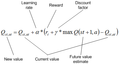
Q values are updated for each state–action pair as an action is selected for a given state. The Q value for the state–action pair is updated with some reward provided by the move (may be nothing) along with the maximum Q value available for the new state reached by applying the action to the current state (discounted by a discount factor). This is further discounted by a learning rate that determines how valuable new information is over old. The discount factor indicates how important future rewards are over short-term rewards. Note that the environment may be filled with negative and positive rewards, or only the goal state may indicate a reward.
Figure 9. A typical Q-learning algorithm
This algorithm is performed over many epochs of reaching the goal state, permitting the Q values to be updated based on the probabilistic selection of actions for states. When complete, the Q values can be used greedily (use the action with the largest Q value for a given state) to exploit the knowledge gained so that the goal state is reached optimally.
Reinforcement learning includes other algorithms that have different characteristics. State-action-reward-state-action is similar to Q-learning except that the selection of an action isn’t based on the maximum Q value but rather includes some probability. Reinforcement learning is an ideal algorithm that can learn how to make decisions in an uncertain environment.
Going further
Machine-learning benefits from a diverse set of algorithms that suit different needs. Supervised learning algorithms learn a mapping function for a data set with an existing classification, where unsupervised learning algorithms can categorize an unlabeled data set based on some hidden features in the data. Finally, reinforcement learning can learn policies for decision-making in an uncertain environment through iterative exploration of that environment.
Ready to go deeper? Take a look at the Get started with machine learning series to understand the principles of machine learning and get working knowledge of the different phases and tasks.
No comments:
Post a Comment