Comparative Study on Classic Machine learning Algorithms

 Machine learning is a scientific technique where the computers learn how to solve a problem, without explicitly program them. Deep learning is currently leading the ML race powered by better algorithms, computation power and large data. Still ML classical algorithms have their strong position in the field.

I will be doing a comparative study over different machine learning supervised techniques like Linear Regression, Logistic Regression, K nearest neighbors and Decision Trees in this story. In the next story, I’ll be covering Support Vector machine, Random Forest and Naive Bayes. There are so many better blogs about the in-depth details of algorithms, so we will only focus on their comparative study. We will look into their basic logic, advantages, disadvantages, assumptions, effects of co-linearity & outliers, hyper-parameters, mutual comparisons etc.

please refer Part-2 of this series for remaining algorithms.

1. Linear Regression

If you want to start machine learning, Linear regression is the best place to start. Linear Regression is a regression model, meaning, it’ll take features and predict a continuous output, eg : stock price,salary etc. Linear regression as the name says, finds a linear curve solution to every problem.

Basic Theory :

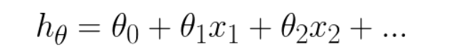
LR allocates weight parameter, theta for each of the training features. The predicted output(h(θ)) will be a linear function of features and θ coefficients.

linear regression output. Eqn (1)

During the start of training, each theta is randomly initialized. But during the training, we correct the theta corresponding to each feature such that, the loss (metric of the deviation between expected and predicted output) is minimized. Gradient descend algorithm will be used to align the θ values in the right direction. In the below diagram, each red dots represent the training data and the blue line shows the derived solution.

gif credits : https://medium.com/@kabab/linear-regression-with-python-d4e10887ca43

Loss function :

In LR, we use mean squared error as the metric of loss. The deviation of expected and actual outputs will be squared and sum up. Derivative of this loss will be used by gradient descend algorithm.

Advantages :

• Easy and simple implementation.
• Space complex solution.
• Fast training.
• Value of θ coefficients gives an assumption of feature significance.

Disadvantages :

• Applicable only if the solution is linear. In many real life scenarios, it may not be the case.
• Algorithm assumes the input residuals (error) to be normal distributed, but may not be satisfied always.
• Algorithm assumes input features to be mutually independent(no co-linearity).

Hyperparameters :

• Regularization parameter (λ) : Regularization is used to avoid over-fitting on the data. Higher the λ, higher will be regularization and the solution will be highly biased. Lower the λ, solution will be of high variance. An intermediate value is preferable.
• learning rate (α) : it estimates, by how much the θ values should be corrected while applying gradient descend algorithm during training. α should also be a moderate value.

Assumptions for LR :

• Linear relationship between the independent and dependent variables.
• Training data to be homoskedastic, meaning the variance of the errors should be somewhat constant.
• Independent variables should not be co-linear.

Colinearity & Outliers :

Two features are said to be colinear when one feature can be linearly predicted from the other with somewhat accuracy.

• colinearity will simply inflate the standard error and causes some significant features to become insignificant during training. Ideally, we should calculate the colinearity prior to training and keep only one feature from highly correlated feature sets.

Outlier is another challenge faced during training. They are data-points that are extreme to normal observations and affects the accuracy of the model.

• outliers inflates the error functions and affects the curve function and accuracy of the linear regression. Regularization (especially L1 ) can correct the outliers, by not allowing the θ parameters to change violently.
• During Exploratory data analysis phase itself, we should take care of outliers and correct/eliminate them. Box-plot can be used for identifying them.

Comparison with other models :

As the linear regression is a regression algorithm, we will compare it with other regression algorithms. One basic difference of linear regression is, LR can only support linear solutions. There are no best models in machine learning that outperforms all others(no free Lunch), and efficiency is based on the type of training data distribution.

LR vs Decision Tree :

• Decision trees supports non linearity, where LR supports only linear solutions.
• When there are large number of features with less data-sets(with low noise), linear regressions may outperform Decision trees/random forests. In general cases, Decision trees will be having better average accuracy.
• For categorical independent variables, decision trees are better than linear regression.
• Decision trees handles colinearity better than LR.

LR vs SVM :

• SVM supports both linear and non-linear solutions using kernel trick.
• SVM handles outliers better than LR.
• Both perform well when the training data is less, and there are large number of features.

LR vs KNN :

• KNN is a non -parametric model, whereas LR is a parametric model.
• KNN is slow in real time as it have to keep track of all training data and find the neighbor nodes, whereas LR can easily extract output from the tuned θ coefficients.

LR vs Neural Networks :

• Neural networks need large training data compared to LR model, whereas LR can work well even with less training data.
• NN will be slow compared to LR.
• Average accuracy will be always better with neural networks.

2. Logistic Regression

Just like linear regression, Logistic regression is the right algorithm to start with classification algorithms. Eventhough, the name ‘Regression’ comes up, it is not a regression model, but a classification model. It uses a logistic function to frame binary output model. The output of the logistic regression will be a probability (0≤x≤1), and can be used to predict the binary 0 or 1 as the output ( if x<0.5, output= 0, else output=1).

Basic Theory :

Logistic Regression acts somewhat very similar to linear regression. It also calculates the linear output, followed by a stashing function over the regression output. Sigmoid function is the frequently used logistic function. You can see below clearly, that the z value is same as that of the linear regression output in Eqn(1).

The h(θ) value here corresponds to P(y=1|x), ie, probability of output to be binary 1, given input x. P(y=0|x) will be equal to 1-h(θ).

when value of z is 0, g(z) will be 0.5. Whenever z is positive, h(θ) will be greater than 0.5 and output will be binary 1. Likewise, whenever z is negative, value of y will be 0. As we use a linear equation to find the classifier, the output model also will be a linear one, that means it splits the input dimension into two spaces with all points in one space corresponds to same label.

The figure below shows the distribution of a sigmoid function.

sigmoid function Eqn(3)

Loss function :

We can’t use mean squared error as loss function(like linear regression), because we use a non-linear sigmoid function at the end. MSE function may introduce local minimums and will affect the gradient descend algorithm.

So we use cross entropy as our loss function here. Two equations will be used, corresponding to y=1 and y=0. The basic logic here is that, whenever my prediction is badly wrong, (eg : y’ =1 & y = 0), cost will be -log(0) which is infinity.

cross-entropy loss Eqn(4)

In the equation given, m stands for training data size, y’ stands for predicted output and y stands for actual output.

Advantages :

• Easy, fast and simple classification method.
• θ parameters explains the direction and intensity of significance of independent variables over the dependent variable.
• Can be used for multiclass classifications also.
• Loss function is always convex.

Disadvantages :

• Cannot be applied on non-linear classification problems.
• Proper selection of features is required.
• Good signal to noise ratio is expected.
• Colinearity and outliers tampers the accuracy of LR model.

Hyperparameters :

Logistic regression hyperparameters are similar to that of linear regression. Learning rate(α) and Regularization parameter(λ) have to be tuned properly to achieve high accuracy.

Assumptions of LR :

Logistic regression assumptions are similar to that of linear regression model. please refer the above section.

Comparison with other models :

Logistic regression vs SVM :

• SVM can handle non-linear solutions whereas logistic regression can only handle linear solutions.
• Linear SVM handles outliers better, as it derives maximum margin solution.
• Hinge loss in SVM outperforms log loss in LR.

Logistic Regression vs Decision Tree :

• Decision tree handles colinearity better than LR.
• Decision trees cannot derive the significance of features, but LR can.
• Decision trees are better for categorical values than LR.

Logistic Regression vs Neural network :

• NN can support non-linear solutions where LR cannot.
• LR have convex loss function, so it wont hangs in a local minima, whereas NN may hang.
• LR outperforms NN when training data is less and features are large, whereas NN needs large training data.

Logistic Regression vs Naive Bayes :

• Naive bayes is a generative model whereas LR is a discriminative model.
• Naive bayes works well with small datasets, whereas LR+regularization can achieve similar performance.
• LR performs better than naive bayes upon colinearity, as naive bayes expects all features to be independent.

Logistic Regression vs KNN :

• KNN is a non-parametric model, where LR is a parametric model.
• KNN is comparatively slower than Logistic Regression.
• KNN supports non-linear solutions where LR supports only linear solutions.
• LR can derive confidence level (about its prediction), whereas KNN can only output the labels.

3. K-nearest neighbors

K-nearest neighbors is a non-parametric method used for classification and regression. It is one of the most easy ML technique used. It is a lazy learning model, with local approximation.

Basic Theory :

The basic logic behind KNN is to explore your neighborhood, assume the test datapoint to be similar to them and derive the output. In KNN, we look for k neighbors and come up with the prediction.

In case of KNN classification, a majority voting is applied over the k nearest datapoints whereas, in KNN regression, mean of k nearest datapoints is calculated as the output. As a rule of thumb, we selects odd numbers as k. KNN is a lazy learning model where the computations happens only runtime.

image credits : https://www.fromthegenesis.com/pros-and-cons-of-k-nearest-neighbors/

In the above diagram yellow and violet points corresponds to Class A and Class B in training data. The red star, points to the testdata which is to be classified. when k = 3, we predict Class B as the output and when K=6, we predict Class A as the output.

Loss function :

There is no training involved in KNN. During testing, k neighbors with minimum distance, will take part in classification /regression.

Advantages :

• Easy and simple machine learning model.
• Few hyperparameters to tune.

Disadvantages :

• k should be wisely selected.
• Large computation cost during runtime if sample size is large.
• Proper scaling should be provided for fair treatment among features.

Hyperparameters :

KNN mainly involves two hyperparameters, K value & distance function.

• K value : how many neighbors to participate in the KNN algorithm. k should be tuned based on the validation error.
• distance function : Euclidean distance is the most used similarity function. Manhattan distance, Hamming Distance, Minkowski distance are different alternatives.

Assumptions :

• There should be clear understanding about the input domain.
• feasibly moderate sample size (due to space and time constraints).
• colinearity and outliers should be treated prior to training.

Comparison with other models :

A general difference between KNN and other models is the large real time computation needed by KNN compared to others.

KNN vs naive bayes :

• Naive bayes is much faster than KNN due to KNN’s real-time execution.
• Naive bayes is parametric whereas KNN is non-parametric.

KNN vs linear regression :

• KNN is better than linear regression when the data have high SNR.

KNN vs SVM :

• SVM take cares of outliers better than KNN.
• If training data is much larger than no. of features(m>>n), KNN is better than SVM. SVM outperforms KNN when there are large features and lesser training data.

KNN vs Neural networks :

• Neural networks need large training data compared to KNN to achieve sufficient accuracy.
• NN needs lot of hyperparameter tuning compared to KNN.

4. Decision Tree

Decision tree is a tree based algorithm used to solve regression and classification problems. An inverted tree is framed which is branched off from a homogeneous probability distributed root node, to highly heterogeneous leaf nodes, for deriving the output. Regression trees are used for dependent variable with continuous values and classification trees are used for dependent variable with discrete values.

Basic Theory :

Decision tree is derived from the independent variables, with each node having a condition over a feature.The nodes decides which node to navigate next based on the condition. Once the leaf node is reached, an output is predicted. The right sequence of conditions makes the tree efficient. entropy/Information gain are used as the criteria to select the conditions in nodes. A recursive, greedy based algorithm is used to derive the tree structure.

credits : https://brookewenig.github.io

In the above diagram, we can see a tree with set of internal nodes(conditions) and leaf nodes with labels( decline/accept offer).

Algorithm to select conditions :

• for CART(classification and regression trees), we use gini index as the classification metric. It is a metric to calculate how well the datapoints are mixed together.

the attribute with maximum gini index is selected as the next condition, at every phase of creating the decision tree. When set is unequally mixed, gini score will be maximum.

• For Iterative Dichotomiser 3 algorithm, we use entropy and information gain to select the next attribute. In the below equation, H(s) stands for entropy and IG(s) stands for Information gain. Information gain calculates the entropy difference of parent and child nodes. The attribute with maximum information gain is chosen as next internal node.

Advantages :

• No preprocessing needed on data.
• No assumptions on distribution of data.
• Handles colinearity efficiently.
• Decision trees can provide understandable explanation over the prediction.

Disadvantages :

• Chances for overfitting the model if we keep on building the tree to achieve high purity. decision tree pruning can be used to solve this issue.
• Prone to outliers.
• Tree may grow to be very complex while training complicated datasets.
• Looses valuable information while handling continuous variables.

Hyperparameters :

Decision tree includes many hyperparameters and I will list a few among them.

• criterion : which cost function for selecting the next tree node. Mostly used ones are gini/entropy.
• max depth : it is the maximum allowed depth of the decision tree.
• minimum samples split : It is the minimum nodes required to split an internal node.
• minimum samples leaf : minimum samples that are required to be at the leaf node.

Comparison with other Models :

Decision tree vs Random Forest :

• Random Forest is a collection of decision trees and average/majority vote of the forest is selected as the predicted output.
• Random Forest model will be less prone to overfitting than Decision tree, and gives a more generalized solution.
• Random Forest is more robust and accurate than decision trees.

Decision tree vs KNN :

• Both are non-parametric methods.
• Decision tree supports automatic feature interaction, whereas KNN cant.
• Decision tree is faster due to KNN’s expensive real time execution.

Decision tree vs naive Bayes :

• Decision tree is a discriminative model, whereas Naive bayes is a generative model.
• Decision trees are more flexible and easy.
• Decision tree pruning may neglect some key values in training data, which can lead the accuracy for a toss.

Decision tree vs neural network :

• Both finds non-linear solutions, and have interaction between independent variables.
• Decision trees are better when there is large set of categorical values in training data.
• Decision trees are better than NN, when the scenario demands an explanation over the decision.
• NN outperforms decision tree when there is sufficient training data.

Decision tree vs SVM :

• SVM uses kernel trick to solve non-linear problems whereas decision trees derive hyper-rectangles in input space to solve the problem.
• Decision trees are better for categorical data and it deals colinearity better than SVM.

In the next story I will be covering the remaining algorithms like, naive bayes, Random Forest and Support Vector Machine.If you have any suggestions or corrections, please give a comment.

Happy Learning :)